Predictive Modelling

Predictive Modelling on AFL Player Disposals

This project aims to predict each player’s number of disposals in every AFL match for the 2023 season. Historical AFL data will be collected and used to create various features. These features will then be used to create a predictive machine learning model.

The project has two goals:

- to see how close on average the model can predict a player's number of disposals in a given match; and
- to use these predictions to bet on the line offered by various betting agencies to see if the model predictions are profitable when used with a betting strategy. Further context on betting is provided below.

Preparing the Data

The fitzRoy package contains functions that allow for processing, cleaning and transforming the data into specific formats that can be used for data analysis. The data was checked for any errors, inconsistencies or missing values prior to exploring it further. This data will ultimately be trained and fed into our machine learing model, so it was important to confirm that it was of high quality before undertaking any further analysis.

Exploring the Data

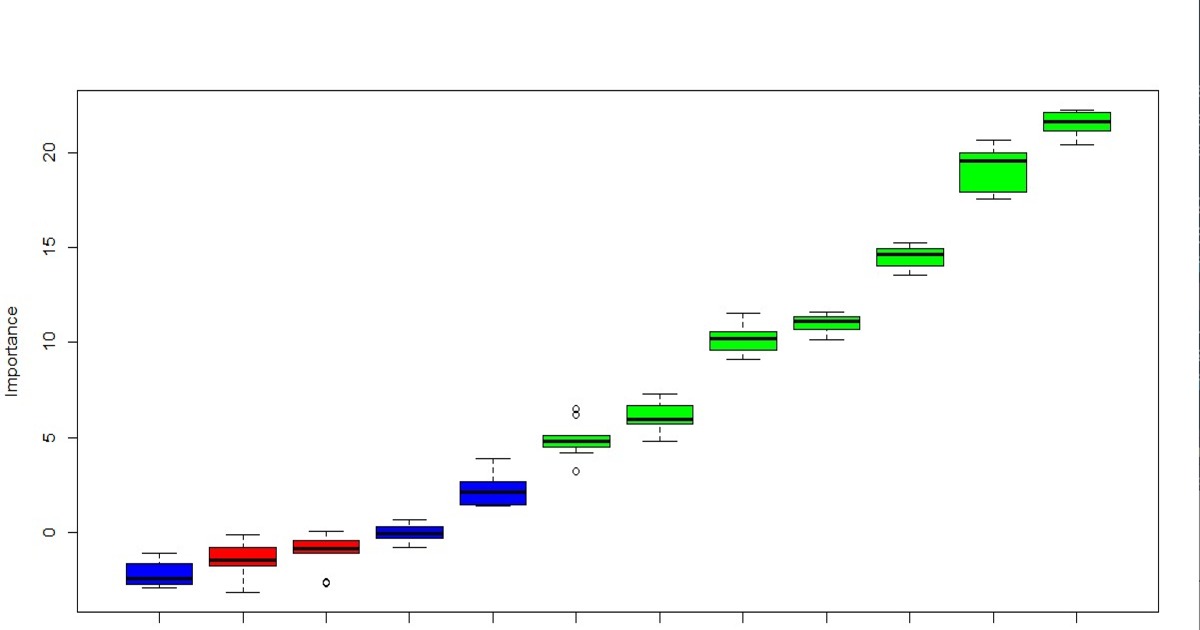
After cleaning and transforming the data, the challenge was to understand what variables would be informative and worthy of including in my model. To that end, I performed an exploratory data analysis, until a number of features were selected for the model based on their importance. The Boruta package was used as a feature slection algortithm, as it captures all features which are in some circumstances relevant to the outcome variable. The confirmed attributes are shown below, along with their mean imprortance.

Feature	meanImp	Decision
Feature 1	21.537022	Confirmed
Feature 2	19.252843	Confirmed
Feature 3	14.549876	Confirmed
Feature 4	11.035390	Confirmed
Feature 5	10.095227	Confirmed
Feature 6	6.073709	Confirmed
Feature 7	4.889339	Confirmed

Our feature selection has provided a clear picture on the signficance of certain variables in our data set. Now, we'll plot the variable importance chart.

Blue box plots correspond to the minimal, average and maximum Z-score of an attrribute. Red and green box plots represent Z-scores of rejected and confirmed attributes respecitvely.

Testing Phase

Now we have our model which we can use to predict player disposals. Most betting agencies will offer a market for each game in every round that will include a number of different players. They will set a line for each player (number of disposals), and the odds for the line. An example of this is as follows:

Rd No.	Match	Player	Line Over	Odds Over	Line Under	Odds Under
12	Melbourne v Sydney	Clayton Oliver	31.5	$1.90	-31.5	$1.88
12	Melbourne v Sydney	Jack Viney	27.5	$1.89	-27.5	$1.88
12	Melbourne v Sydney	Callum Mills	24.5	$1.92	-24.5	$1.79

If our model predicts that Clayton Oliver will have a total of 30 disposals for the match, Jack Viney 28 disposals and Callum Mills 21 disposals, then we would bet on the line under, over and under respecitvely, like so:

Rd No.	Match	Player	Line Over	Odds Over	Line Under	Odds Under	Pred. Disposals	Bet Type
12	Melbourne v Sydney	Clayton Oliver	31.5	$1.90	-31.5	$1.88	30	Under
12	Melbourne v Sydney	Jack Viney	27.5	$1.89	-27.5	$1.88	28	Over
12	Melbourne v Sydney	Callum Mills	24.5	$1.92	-24.5	$1.9	21	Under

The model was tested over the first six rounds of the 2023 season, producing strong results, with an average strike rate of 56%. This means that more than half the time, the model is correctly predicting whether or not the number of player disposals will fall under or over the line offered. But what does this mean when we start to apply this to real world bets? Break even is generally considered to be around 52-53% (depending on the bookie's market percentage), so with an average strike rate of 56%, we are well ahead of the market and therefore our model is profitable.

Betting Strategy

How do we know our model is profitable? Profit in betting is generally referred to as Profit on Turnover or PoT as it is more commonly known. We can use a very simple formula to convert our strike rate into PoT:

PoT = (Strike Rate x Price) - 1

We know that our strike rate during the testing phase was 56%. Our average price was $1.88, so we calculate our PoT as follows:

PoT = (0.56 x 1.88) - 1

PoT = 5.28%

Model Implementation

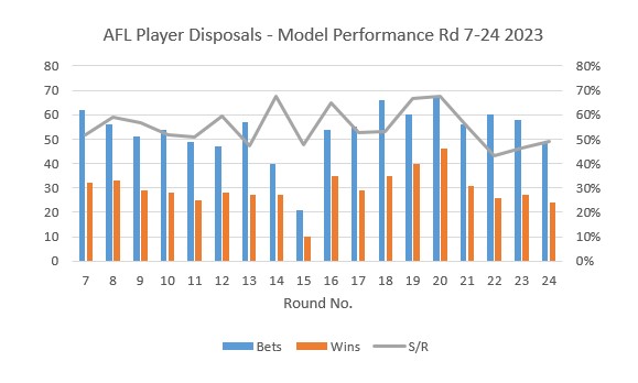
After testing was completed on rounds 1-6, the model was then put into real-time use to see how it would perform for the remainer of the season. The average strike rate from round 6 to round 24 was 56%. This is consistent with the strike rate produced during the testing phase of rounds 1-6 (56%), and our model remains profitable.

Betting Results

We can verify that our model is profitable by looking at a summary of the betting performance. We know our strike rate was a solid 56%, and the average price remained at $1.88 through the rest of the season. We can verify our PoT again using the formula shown above:

PoT = (0.56 x 1.88) - 1

PoT = 5.28%

Bets	Wins	Strike Rate	Profit	PoT
1410	789	56%	78.9	5.6%

At $100 per unit, the model produced a profit of over 78 units or $7,800 profit for the entire season! Note that the PoT shown above (5.6%) differs slightly from the result of our formula (5.28%) as the average price was closer to $1.89 for the season when accounting for rounding.

Model and Betting Aids

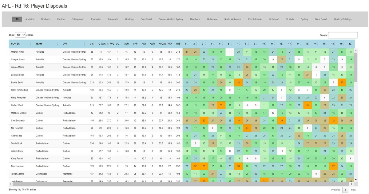
In order to verify our model predictions and to assist with the overall betting strategy, I produced an interactive chart in Shiny that is prepared prior to each game. It provides an overall snapshot of some of the more key components, including a heat map of previous disposals. The chart is designed to aid in making the right betting decisions.

You can see the full analysis and model in my GitHub repository here.